-
Insertion Sort
1. Strategy
- 원소를 적절한 순서대로 삽입(Insertion)한다.
- 첫 번째 원소는 정렬된 상태이다.
- 임의의 원소 $x$를 꺼낸다.
- $x$의 적절한 위치를 찾을 때까지 계속해서 배열의 원소들과 비교한다.
- 이를 모든 원소가 정렬될 때까지 반복한다.
2. Algorithm
- 입력값 : 정렬되지 않은 배열
- 출력값 : 오름차순으로 정렬된 배열
void insertionSort(Element[] E, int n)
	int xIndex;
	for (xIndex = 1; xIndex < n; xIndex++)
		Element current = E[xIndex];
		Key x = current.key;
		int xLoc = shiftVacRec(E, xIndex, x);
		E[xLoc] = current
	return;

int shitfVacRec(Element[] E, int vacant, Key x)
	int xLoc;
	if (vacant == 0)
		xLoc = vacant;
	else if (E[vacant - 1].key <= x)
		xLoc = vacant;
	else
		E[vacant] = E[vacant - 1];
		xLoc = shiftVacRec(E, vacant - 1, x);
	return xLoc;
3. Analysis
- Worst-Case Complexity
- 입력이 역순인 경우 : $W(n)=\sum_{i=1}^{n-1}i = n(n-1) \ / \ 2 \in \Theta(n^2)$
- Best-Case Complexity
- 입력이 정렬되있는 경우 : $B(n) \in \Theta (n)$
- Average Behavior
- $A_{fail}(i) = i \ / \ (i + 1) = 1 - 1 \ / \ (i + 1)$
- $A_{succ}(i) = 1 \ / \ (i + 1) \times \sum_{j=1}^i j = i \ / \ 2$
- $A(n)=\sum_{i=1}^{n-1}(A_{fail}(i)+A_{succ}(i)) \approx n^2 \ / \ 4 \in \Theta(n^2)$
- Optimality
- 인접한 두 원소를 비교하는 알고리즘 중에선 최적 알고리즘이다.
- 다만 정렬 알고리즘으로는 최적 알고리즘이 아니다.
Quick Sort
1. Strategy
- Divide-and-Conquer(분할 정복)에 기반한 임의의 원소를 선택하는 로직이다.
- Divide (분할) : 임의의 원소 $x$를 선택하고 구간을 나눈다.
- $L$ : $x$보다 작은 원소들
- $E$ : $x$와 같은 원소들
- $G$ : $x$보다 큰 원소들
- Conquer (정복) : $L$과 $G$를 정렬한다.
- Combine (병합) : $L$, $E$, 그리고 $G$를 합친다.
2. Algorithm
- 입력값 : 일렬의 원소들 $S$, 피벗의 위치 $p$
- 출력값 : 일렬의 원소들 $L$, $E$, $G$
partition(S, p)
	L, E, G ← empty sequences;
	x ← S.remove(p);
	while ¬S.isEmpty()
		y ← S.remove(S.first());
		if y < x
			L.insertLast(y);
		else if y = x
			E.insertLast(y);
		else {y > x}
			G.insertLast(y);
	return L, E, G;
3. Analysis
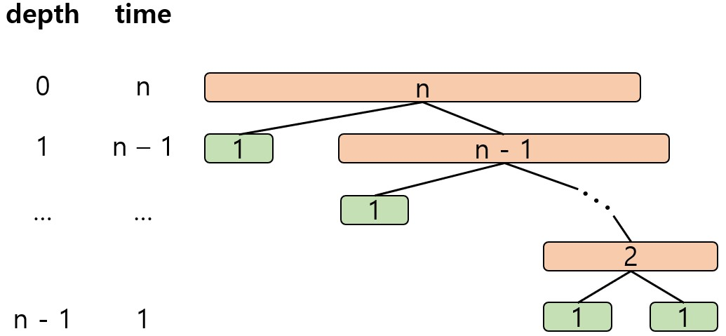
- Worst-Case
- 피벗이 가장 큰, 또는 가장 작은 원소일 경우
- Running Time : $n + (n-1) + \cdots + 2 + 1 \approx O(n^2)$
- Average Behaviour : $A(n) \in O(n \log{n})$
Worst-Case에서 Quick Sort 4. Quick Sort 구현 (In-Place Quick Sort)
- 인덱스 두 개를 통해 $S$를 $L$과 $E \cup G$ 두 개의 배열로 나눈다.
- $h$와 $k$가 교차할 때까지 반복한다. ($h$ : $L$의 기준, $k$ : $E \cup G$의 기준)
- 입력값 : 일렬의 원소들 $S$, 인덱스 $l$, $r$
- 출력값 : 오름차순으로 정렬된 배열 $S$
inPlaceQuickSort(S, l, r)
	if l >= r
		return;
	i ← a random integer between l and r;
	x ← S.elemAtRank(i);
	(h, k) ← inPlacePartition(x);
	inPlaceQuickSort(S, l, h - 1);
	inPlaceQuickSort(S, k + 1, r);
Merge Sort
1. Strategy
- Divide : 입력 배열을 같은 크기의 2개의 부분 배열로 분할
- Conquer : 부분 배열을 정렬 -> 원소의 갯수가 1개일 경우 정렬된 상태
- Combine : 정렬된 부분 배열들을 하나의 배열에 합병 -> Merging Sorted Sequence
2. Merging Sorted Sequences
- Problem : 오름차순으로 정렬된 두 배열을 하나로 합친다.
- Strategy
- $A$ 배열과 $B$ 배열에 첫번째 원소에 인덱스를 각각 설정한다.
- 인덱스의 값을 비교하여 $C$ 배열에 추가한다.
- 두 인덱스 중 하나라도 배열의 끝에 도달했다면, 나머지 배열의 모든 값은 그대로 $C$ 배열에 붙여준다.
- Analysis
- Worst-Case : $n-1 \in O(n)$
- Best-Case : $n \ / \ 2 \in O(n)$
Merge(A, B, C)
	if A is empty
		rest of C = rest of B;
		return;
	else if B is empty
		rest of C = rest of A;
		return;
	else if first of A <= first of B
		first of C = first of A;
		merge(rest of A, B, rest of C);
	else
		first of C = first of B;
		merge(A, rest of B, rest of C);
3. Algorithm
- 입력값 : 배열 $E$와 첫번째, 마지막 인덱스
- 결과값 : 정렬된 배열 $E$
void mergeSort(Element[] E, int first, int last)
	if (first < last)
		int mid = (first + last) / 2;
		mergeSort(E, first, mid);
		mergeSort(E, mid + 1, last);
		merge(E, first, mid, last);
	return;
4. Analysis
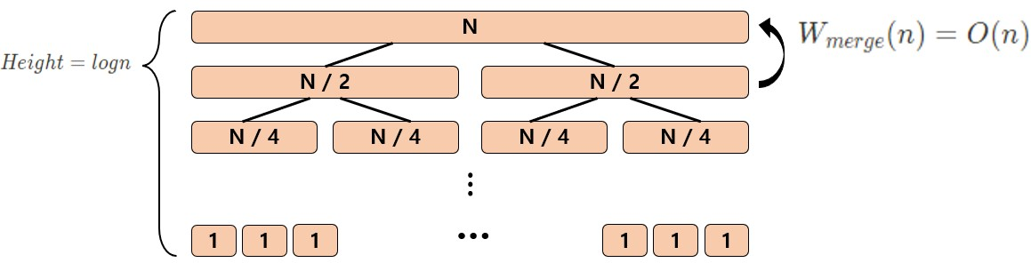
- $W(n) = W(n \ / \ 2) + W(n \ / \ 2) + W_{merge}(n) \in \Theta (n \log{n})$
- Optimal : 원소끼리 대소를 비교하여 정렬하는 알고리즘 중엔 최적
Merge Sort의 Sequence Heap Sort
1. Strategy
- Heap 데이터 구조에 원소들을 넣는다.
- Root 노드의 원소를 반복적으로 제거할 필요가 있다, -> 총 N번의 delete 연산이 필요.
2. Algorithm
- Construct Heap
void constructHeap(H) if H is not a leaf constructHeap(left subtree of H); constructHeap(right subtree of H); Element K = root(H); fixHeap(H, K); return;- Heap Sort
- fixHeap은 $2h$만큼의 비교 연산이 필요하다.
- $W(n) \approx 2\log{n} \in O(\log{n})$
heapSort(E, n)
	constructHeap(E); // construct H from E
	for i from n to 1
		curMax = getMax(H);
		deleteMax(H);
		E[i] = curMax;

deleteMax(H) // Structure property
	copy the rightmost element of the lowest level of H into K
	delete the element
	fixHeap(H, K)

fixHeap(H, K) // Order property, Down-Heap
	if H is a leaf
		insert K in root(H)
	else
		set largerSubHeap
		if K.key >= root(largerSubHeap.key)
			insert K in root(H);
		else
			insert root(largerSubHeap) in root(H);
			fixHeap(largerSubHeap, K);
	return;
3. Analysis
- Heap 데이터 구조 설계 + Root 노드 제거 ($1 ~ n$)
- $O(n) + 2n\log{n} \in O(n\log{n})$
Accelerated Heap Sort
1. Strategy
- Root 노드를 제거한 후 Heap 데이터 구조를 수정할 때 Depth를 1씩 내려가는 것이 아닌 $h$의 절반만큼 내려간다.
- 절반만큼 내려왔을때 해당 노드가 올바른 위치가 아닐 경우 부모 노드와 크기를 비교한다.
- 위로 올라가는 경우 버블 정렬을 사용한다.
- 아래로 내려가는 경우 재귀적으로 남은 높이의 절반만큼 내려간다.
2. Algorithm
void fixHeapFast(Element[] E, int n, Element K, int vacant, int h)
	if h <= 1
		Process heap of height 0 or 1
	else
		int hStop = h / 2;
		int vacStop = promote(E, hStop, vacant, h);
		// vacStop is new vacant location, at height hStop
		int vacParent = vacStop / 2;
		if E[vacParent].key <= K.key
			E[vacStop] = E[vacParent];
			bubbleUpHeap(E, vacant, K, vacParent);
		else
			fixHeapFast(E, n, K, vacStop, hStop);

// 자식 노드들을 비교하며 hStop까지 내려가는 함수
int promote(Element[] E, int hStop, int vacant, int h)
	int vacStop;
	if h <= hStop;
		vacStop = vacant;
	else if E[2 * vacant].key <= E[2*vacant + 1].key
		E[vacant] = E[2*vacant + 1];
		vacStop = promote(E, hStop, 2 * vacant + 1, h - 1);
	else
		E[vacant] = E[2 * vacant];
		vacStop = promote(E, hStop, 2 * vacant, h - 1);
	return vacStop;

// 잘못 내려왔을 때 K의 옳바른 위치를 찾아 올라가는 함수
void bubbleUpHeap(Element[] E, int root, Element K, int vacant)
		if vacant == root
			E[vacant] = K;
		else
			int parent = vacant / 2;
			if K.key <= E[parent].key
				E[vacant] = K;
			else
				E[vacant] = E[parent];
				bubbleUpHeap(E, root, K, parent);
3. Analysis
- Worst-Case : bubbleUpHeap 함수가 호출되지 않는 경우, 즉 Leaf 노드까지 도달한 경우
- fixHeapFast의 비교 횟수 : $h \ / \ 2 + 1 + h \ / \ 4 + 1 + h \ / \ 8 + 1 + \cdots \approx h + \log{h}$
- $W(n) = n(\log{n} + \log{(\log{n})}) \in O(n\log{n})$
Radix Sort
지금까지의 정렬 알고리즘의 기본 연산은 두 원소의 비교 연산이였다. 이를 다른 연산으로 바꿔서 정렬을 한다면 알고리즘의 성능은 달라질 수 있다.
1. Strategy
- 마지막 자릿수를 사용하여 여러 Buckets으로 분할
- 각 Buckets을 정렬
- 정렬된 Buckets을 병합
2. Algorithm
List radixSort(List L, int radix, int numFields)
	List[] buckets = new List[radix];
	int field; // field number within the key
	List newL;
	newL = L;
	for each field from 0 to numFields
		Initialize buckets array to empty lists
		distribute(newL, buckets, radix, field);
		newL = combine(buckets, radix);
	return newL;

//distribute keys into buckets
void distribute(List L, List[] buckets, int radix, int field)
	List remL;
	remL = L;
	while remL != nil
		Element K = first(remL);
		int b = maskShift(field, radix, K.key);
		// maskShift(f, r, key) selects field f of key
		buckets[b] = cons(K, buckets[b]); // construct list
		remL = rest(remL);
	return;

//Combine linked lists in all buckets into one list L
List combine(List[] buckets, int radix)
	int b; // bucket number
	List L, remBucket;
	L = nil;
	for each b from radix - 1 to 0
		remBucket = buckets[b];
		while remBucket != nil
			key K = first(remBucket);
			L = cons(K, L);
			remBucket = rest(remBucket);
	return L;
3. Analysis
- Buckets 분할 : $\Theta (n)$
- Buckets 병합 : $\Theta (n)$
- 자릿 수 : $d$ (constant)
- 시간 : $O(d *n) \approx O(n)$
- 공간 : $O(n)$
Stability in sorting algorithm
같은 키를 가진 두 객체가 정렬 전이나 정렬 후의 순서가 같다면 이를 Stable하다고 한다.
$if \ i < j \ and \ A[i] \equiv A[j], \ then \ \pi (i) < \pi(j) \ after\ sorting$
$\pi (i)$ : 정렬 이후 $i$의 Index
'CS > 알고리즘' 카테고리의 다른 글
String Matching (0) 2023.11.23 Dynamic Programming (0) 2023.11.22 Graph Optimization Problems and Greedy Algorithms (0) 2023.11.22 Graphs and Graph Traversals (0) 2023.11.21 Analyzing Algorithms and Problem Principles (0) 2023.11.13